ViT: An Image is Worth 16×16 Words: Transformers for Image Recognition at Scale

Google Research, Brain Team

The 9th International Conference on Learning Representations, ICLR, 2021.

Introduction

Motivation

The Transformer model and its variants have been successfully shown that they can be comparable to or even better than the state-of-the-art in several tasks, especially in the field of NLP. 

Objective

• Introduce Vision Transformer (ViT), which is applied directly to sequences of image patches by analogy with tokens (words) in NLP. 
• Show that a pure Transformer can perform very well on image classification tasks. 

Related Works

Attention mechanisms

Attention mechanisms improve CNN performance by focusing on relevant features. For example:

• Spatial Attention: Non-local neural networks help CNNs capture long-range pixel dependencies and understand global context.
• Channel Attention: SENet uses squeeze-and-excitation (SE) blocks to improve feature representation by focusing on important channels.

Combining CNNs with Transformers has also proven effective. Detection Transformer (DETR) uses a Transformer to process CNN feature maps for end-to-end object detection, removing the need for hand-designed steps like non-maximal suppression. Similar approaches have been applied to semantic segmentation in models like SETR and Trans2Seg.

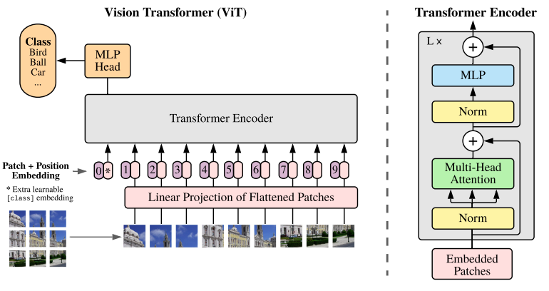
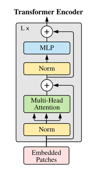
The Transformer encoder in ViT

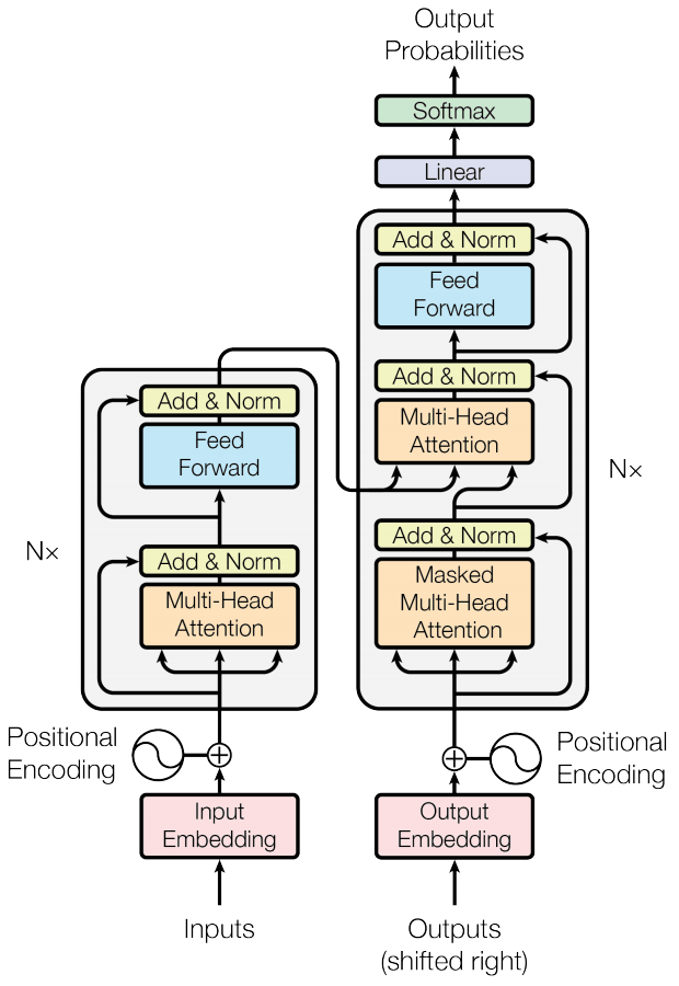
The Vision Transformer (ViT) encoder closely follows the original Transformer architecture by Vaswani et al.

The main difference is that ViT applies layer normalization before the multi-head attention and MLP blocks (pre-norm), unlike the original’s post-norm approach. This pre-norm technique enables more stable and efficient training, especially for deeper models.

For classification, only the output corresponding to the initial classification token is passed to an MLP head to generate the final prediction.

Subsequent models have introduced further improvements:

• DeiT: Employs a knowledge distillation technique to train ViT more effectively.
• CaiT: Explores architectural modifications to the base ViT model.
• T2T-ViT: Proposes a more advanced tokenization process to better represent the input image.

Framework

• A key idea of applying a Transformer to image data is how to convert an input image into a sequence of tokens, which is usually required by a Transformer.
  1. An input image of size H x W is divided into N non-overlapping patches of size 16 x 16 pixels, where N = (H x W) / (16 x 16). 
  2. Each patch is then converted into an embedding using a linear layer. These embeddings are grouped together to construct a sequence of tokens, where each token represents a small part of the input image. 
  3. An extra learnable token, i.e., classification token [CLS], is prepended to the sequence. It is used by the Transformer layers as a place to pull attention from other positions to create a prediction output. 
  4. Positional embeddings are added to this sequence of N + 1 tokens and then fed into a Transformer encoder.

Contribution

Details

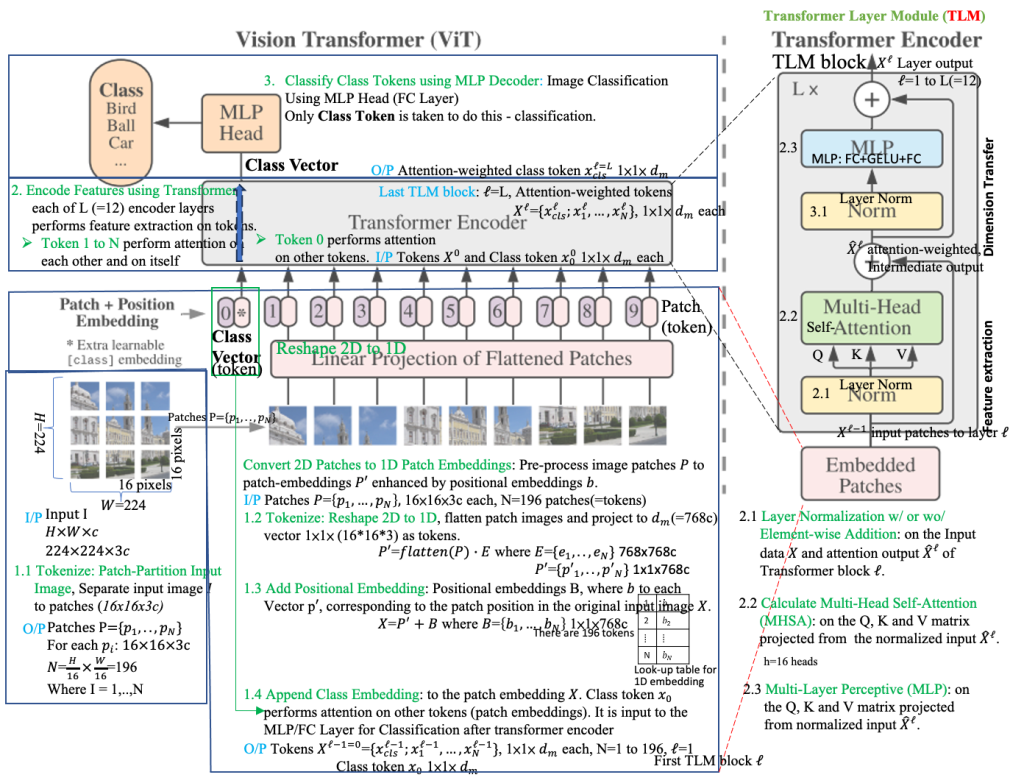
Step 1: Tokenizer – Image to Patches

• Input: An image of a cat, size 224×224 pixels.
• Process: We divide this image into a grid of non-overlapping patches. A common patch size is 16×16 pixels.
• Output: We get a grid of 14×14 patches (since 224 / 16 = 14). Each patch is 16x16x3 (3 for RGB color channels).
• Visualization:
  1. [Original 224×224 Image of a Cat] -> [Grid of 14×14 Patches]

Step 2: Flatten Patches & Linear Projection

• Input: 14×14 = 196 patches, each 16x16x3.
• Process:
  1. Flatten: Each 16x16x3 patch is flattened into a single vector of 16 * 16 * 3 = 768 elements.
  2. Linear. Projection: These 768-dimensional vectors are then projected into a lower-dimensional space (e.g., to 512 dimensions). This is done using a learnable linear transformation (a matrix multiplication). The specific number of dimensions is a hyperparameter called the “embedding dimension” or “model dimension” (often represented as “D”).
• Output: 196 patch embeddings, each a 512-dimensional vector.
• Visualization:
  1. [Patch 1 (16x16x3)] -> [Flatten to 768-D vector] -> [Project to 512-D Patch Embedding]
  2. [Patch 2 (16x16x3)] -> [Flatten to 768-D vector] -> [Project to 512-D Patch Embedding]
  3. …
  4. [Patch 196 (16x16x3)] -> [Flatten to 768-D vector] -> [Project to 512-D Patch Embedding]

Step 3: Add Position Embeddings

• Input: 196 patch embeddings (512-D each).
• Process: We add a unique position embedding to each patch embedding. These position embeddings are also 512-dimensional vectors and are either learned or predefined (e.g., using sinusoidal functions). This step informs the model about the original location of each patch in the image.
• Output: 196 position-aware patch embeddings (512-D each).
• Visualization:
  1. [Patch Embedding 1 (512-D)] + [Position Embedding 1 (512-D)] = [Positional Patch Embedding 1]
  2. [Patch Embedding 2 (512-D)] + [Position Embedding 2 (512-D)] = [Positional Patch Embedding 2]
  3. …
  4. [Patch Embedding 196 (512-D)] + [Position Embedding 196 (512-D)] = [Positional Patch Embedding 196]

Step 4: Prepend Class Token

• Input: 196 position-aware patch embeddings (512-D each).
• Process: We add a special learnable vector called the “[CLS]” token embedding (also 512-D) to the beginning of the sequence.
• Output: A sequence of 197 embeddings: [CLS] + 196 positional patch embeddings. Each embedding is 512-D.
• Visualization:
  1. [CLS Token (512-D)] + [Positional Patch Embedding 1] + [Positional Patch Embedding 2] + … + [Positional Patch Embedding 196]

Step 5: Transformer Encoder

• Input: A sequence of 197 embeddings (512-D each).
• Process: This sequence is fed into the Transformer Encoder, which consists of multiple identical layers stacked on top of each other. Each layer has two main sub-layers (Each sublayer is also followed by Layer Normalization and uses residual connections):
  1. Multi-Head Self-Attention: This mechanism allows the model to weigh the importance of different patches in relation to each other. It calculates attention scores between all pairs of embeddings (including the [CLS] token).
  2. Feed-Forward Network: A simple fully connected network that further processes each embedding individually.
• Output: A sequence of 197 encoded embeddings (512-D each), where each embedding now contains contextual information from other embeddings in the sequence. The [CLS] token embedding, in particular, will contain aggregated information from all patches.
• Visualization (simplified for one Encoder layer):
  1. [Input Sequence (197 x 512-D)] -> [Multi-Head Self-Attention] -> [Feed-Forward Network] -> [Output Sequence (197 x 512-D)]

Step 6: MLP Head (Classification)

• Input: The encoded embedding corresponding to the [CLS] token from the final Transformer Encoder layer (512-D).
• Process: This embedding is passed through a Multi-Layer Perceptron (MLP) head, typically a small neural network with one or more hidden layers, that outputs the final classification probabilities.
• Output: A vector of class probabilities.
• Visualization:
  1. [Encoded [CLS] Token (512-D)] -> [MLP Head] -> [Class Probabilities (e.g., 1000-D)] -> [Prediction: Cat (highest probability)]

Final Output

• The model predicts the class with the highest probability (in this case, “Cat”).

Loss Function

Cross-Entropy Loss

Experimental Results

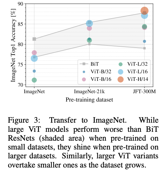
Key Takeaways

According to [2]:

1. A requirement of a large amount of data for pre-training. Unlike CNNs, ViTs (or a typical Transformer-based architecture) do not have well-informed inductive biases (such as convolutions for processing images). ==> DeiT, CaiT, T2T-ViT
2. High computational complexity, especially for dense prediction in high-resolution images. The computational complexity of the attention module, which is quadratic to the image size. ==> PVT, FAVOR+.

According to PVT Paper:

Due to the limited resource, the input of ViT is coarse-grained (e.g., the patch size is 16 or 32 pixels), and thus its output resolution is relatively low (e.g., 16-stride or 32-stride). As a result, it is difficult to directly apply ViT to dense prediction tasks that require high-resolution or multi-scale feature maps.

Reference

• https://keras.io/examples/vision/image_classification_with_vision_transformer/
• Vision Transformers: A Review
  1. https://sertiscorp.medium.com/vision-transformers-a-review-part-i-19153d1f5c3b
  2. https://sertiscorp.medium.com/vision-transformers-a-review-part-ii-a31136cf848d
  3. https://sertiscorp.medium.com/vision-transformers-a-review-part-iii-cd07d699a504
• [12] Learning Deep Transformer Models for Machine Translation https://www.aclweb.org/anthology/P19-1176.pdf
• [13] Adaptive Input Representations for Neural Language Modeling https://openreview.net/pdf?id=ByxZX20qFQ
• H. Touvron, M. Cord, M. Douze, F. Massa, A. Sablayrolles, and H. Jégou, “Training data-efficient image Transformers & distillation through attention,” arXiv Preprint, arXiv2012.12877, 2020. (DeiT)
• H. Touvron, M. Cord, A. Sablayrolles, G. Synnaeve, and H. Jégou, ”Going deeper with image Transformers,” arXiv Preprint, arXiv2103.17329, 2021. (CaiT)
• L. Yuan, Y. Chen, T. Wang, W. Yu, Y. Shi, Z. Jiang, et al., “Tokens-to-token ViT: Training Vision Transformers from scratch on ImageNet,” arXiv Preprint, arXiv2101.11986, 2021. (T2T-ViT)