

This is a summary of the introductory lecture for Stanford’s CS25: Transformers United.
Deep Learning Models that have Revolutionized NLP, CV, RL
The first lecture introduces the instructors, provides a high-level overview of the course, and gives a brief history and explanation of the Transformer architecture.
The Rise of Transformers
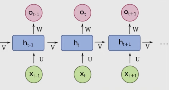
- Pre-Transformer Era: Models like RNNs and LSTMs were used for sequence modeling but struggled with long sequences and capturing context.
- The “Attention Is All You Need” Paper (2017): This paper introduced the Transformer architecture and its core component, the self-attention mechanism.
- Current and Future Applications: Transformers are now used in a wide range of fields, including:
- Protein Folding: AlphaFold
- Text and Image Generation: DALL-E, GPT-3
- Reinforcement Learning
- Potential future applications in video understanding and finance.
Key Components of Transformers
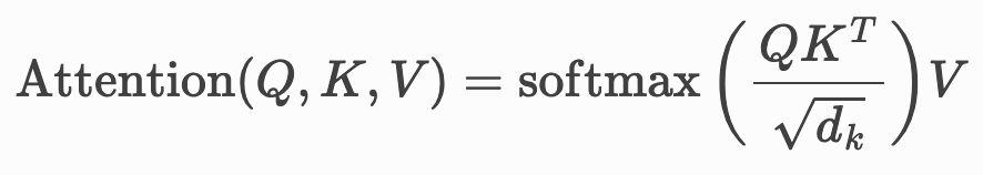
- Self-Attention: The central idea is a search-retrieval mechanism where for a given query (a token), the model finds the most similar keys (other tokens) and returns their corresponding values. This allows every token to attend to every other token, capturing rich contextual relationships.

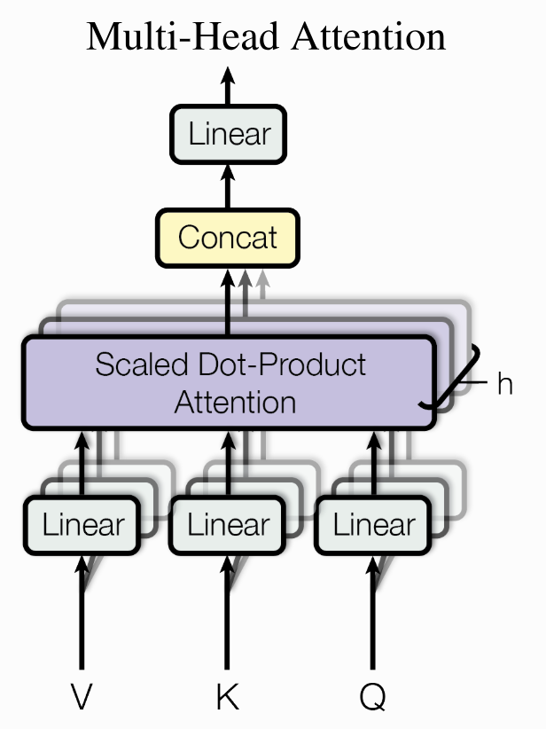
- Multi-Head Attention: The self-attention mechanism is performed multiple times in parallel (“heads”), allowing the model to learn different types of relationships simultaneously (e.g., syntactic structure, part-of-speech).
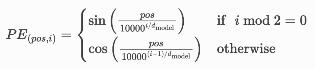
- Positional Encodings: Since self-attention is order-agnostic, these are added to give the model a sense of the position of each token in the sequence.
- Feed-Forward Layers (Nonlinearities): These provide the necessary non-linearity, as self-attention is a linear operation.
- Masking: In the decoder, masking is used to prevent the model from “cheating” by looking at future tokens during training.
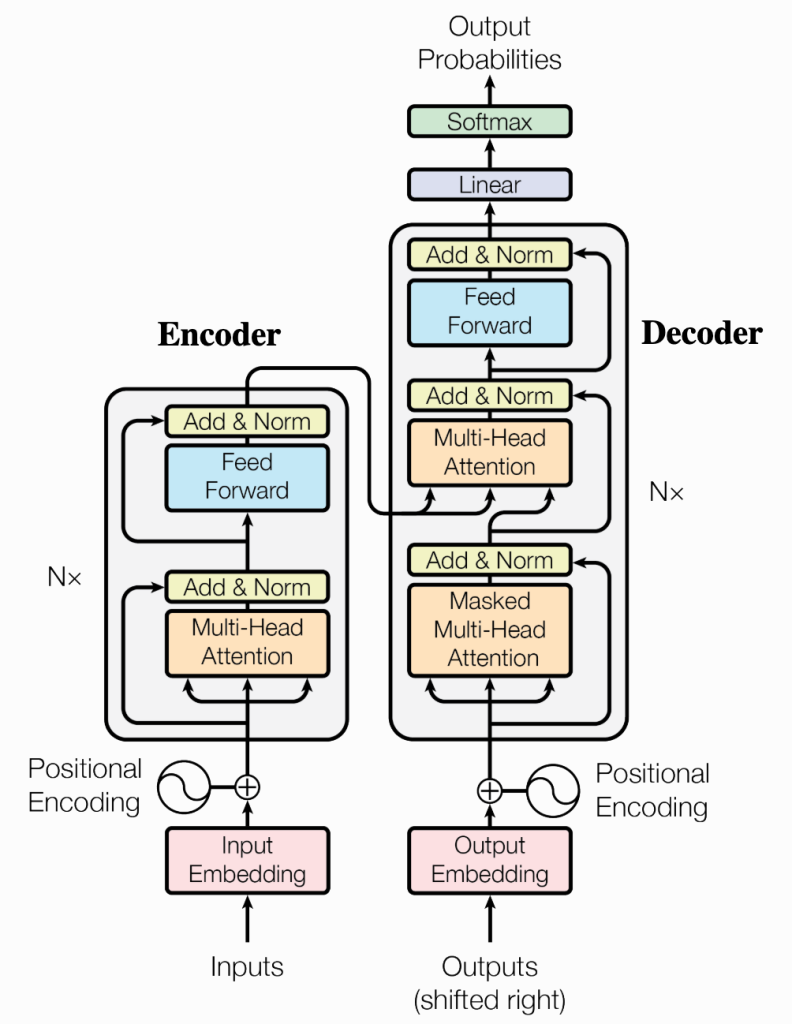
The Encoder-Decoder Architecture
The original Transformer has two main parts:
- Encoder: Reads and encodes the entire input sequence (e.g., an English sentence). Each has:
- A self-attention layer followed by a feedforward layer.
- Each of these is also followed by a layer norm.
- There are residual connections between encoder blocks.
- Decoder: Generates the output sequence token by token (e.g., the French translation), paying attention to both the previously generated tokens and the encoder’s output.
- Similar to Encoder, except that it has a 3rd layer, that performs multi head attention on the output from the encoders.
- Masking is used to prevent positions looking ahead during self-attention.
Advantages and Disadvantages
- Advantages:
- Constant Path Length: The distance between any two tokens is always one, solving the long-range dependency problem of RNNs.
- Parallelization: The computations are highly parallelizable, making them much faster to train on modern hardware like GPUs.
- Disadvantages:
- Quadratic Complexity: Self-attention has a time complexity of O(n²), which is computationally expensive for very long sequences.
- Subsequent works solved this problem: Big Bird, Linformer, Reformer.
Post-Transformer Models: GPT and BERT
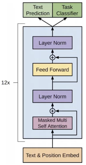
- GPT (Generative Pre-trained Transformer):
- Uses only the decoder blocks.
- Trained on a next-token prediction task.
- Excels at in-context learning (few-shot learning without gradient updates).
- BERT (Bidirectional Encoder Representations from Transformers):
- Uses only the encoder blocks.
- Trained with a Masked Language Modeling objective, where it predicts masked-out words.
- Also uses a Next Sentence Prediction task.
Papers
- Show, Attend and Tell: Neural Image Caption Generation with Visual Attention
- Attention is all you need
- Effective Approaches to Attention-based Neural Machine Translation
- A Structured Self-attentive Sentence Embedding
- Big Bird: Transformers for Longer Sequences
- Linformer: Self-Attention with Linear Complexity
- Reformer: The Efficient Transformer
- Language Models are Few-Shot Learners
- BERT: Pre-training of Deep Bidirectional Transformers for Language Understanding
Transformer in Language: The Development of GPT Models
This lecture provides a historical overview of generative language models, detailing the journey from simple statistical models to the massive, capable Transformers developed at OpenAI like GPT-3 and Codex. The talk emphasizes the shift from supervised learning to a paradigm of unsupervised pre-training followed by task-specific fine-tuning or prompting.
The Evolution of Language Models
The lecture charts the progress in text generation quality through several key stages:
- N-Gram Models (~1951): Produced incoherent gibberish.
- Recurrent Neural Networks (RNNs, ~2011): Generated text with sentence-like flow but no real meaning.
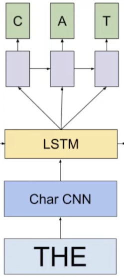
- LSTMs (~2016): Achieved more coherence and could model longer-term dependencies, though still with noticeable artifacts.
- Transformers (GPT-2, ~2019): Capable of generating coherent, multi-paragraph text, even inventing and persisting fictional details.
- GPT-3 (~2020): Reached a level where its generated prose is stylistically consistent and often poetic. As model size increased, humans’ ability to distinguish its generated news articles from real ones dropped to near chance.
Unsupervised Learning: The Core Paradigm
The central motivation behind the GPT series was not just to create good language models, but to leverage unsupervised learning. The key ideas are:
- Leverage the Internet: Use the massive trove of unlabeled text data available online for pre-training.
- Analysis by Synthesis: A model that can effectively create (generate) coherent text must first understand the underlying structure, grammar, and concepts of language.
- Autoregressive Pre-training: The simple objective of “predicting the next word” is surprisingly powerful. To predict the last word of a mystery novel, for example, the model needs a deep understanding of the entire plot.
This approach was first validated by the “Unsupervised Sentiment Neuron” (2017), where an LSTM trained simply to predict the next character in Amazon reviews spontaneously developed a single neuron that corresponded directly to sentiment (positive/negative).
The GPT Series And In-Context Learning
- GPT-1: The first major model to demonstrate that pre-training on internet text and then fine-tuning (updating weights) for specific tasks was a viable and powerful approach.
- GPT-2: Introduced the concept of zero-shot learning. Instead of fine-tuning, tasks could be solved by framing them as a text completion problem. For example, adding “TLDR;” to the end of an article prompts the model to generate a summary.
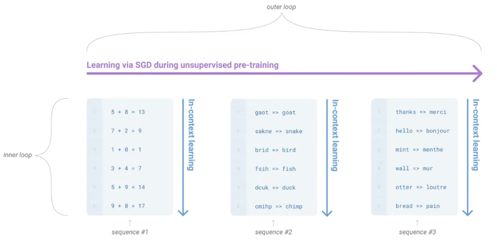
- GPT-3: Advanced this to few-shot or in-context learning. The model can learn a new task at inference time simply by being shown a few examples in the prompt, without any gradient updates. Performance on these tasks was shown to scale directly with model size.
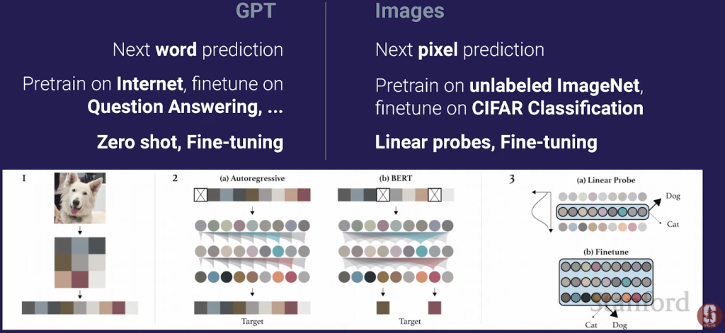
Autoregressive Language Modeling is Universal
The talk argues that the Transformer is a universal sequence model. The same architecture can be applied to any data that can be represented as a sequence of bytes.
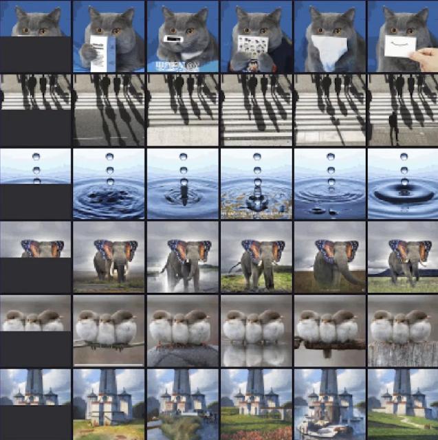
- iGPT: By treating an image as a sequence of pixels, a standard Transformer can be trained for next-pixel prediction. This model, trained without any 2D-specific inductive biases (like convolutions), achieves state-of-the-art results on image classification benchmarks like CIFAR.
- DALL-E: Takes this a step further by training on a sequence of text and image tokens combined. This allows it to generate images from text captions and perform remarkable zero-shot image-to-image transformations, like turning a photo of a cat into a sketch.
Codex: Applying Transformers to Code
This section focuses on Codex, a model fine-tuned from GPT-3 on a massive dataset of public code from GitHub.
- Evaluation is Key: Traditional language metrics like BLEU are poor for evaluating code. A new benchmark, HumanEval, was created with hand-written problems and unit tests to check for functional correctness.
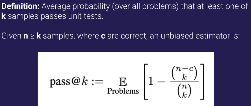
- The Pass@k Metric: To evaluate performance, the
pass@kmetric was introduced. It measures the probability that at least one ofkgenerated samples for a given problem passes the unit tests.
- The Unreasonable Effectiveness of Sampling: The most striking result was the massive performance gap between
pass@1andpass@100. By generating 100 different solutions and checking them, the model’s success rate jumped from under 30% to over 70%. This shows the model isn’t just generating one solution but is exploring a diverse space of functionally different programs. - Further Fine-tuning: Performance was further improved by fine-tuning on high-quality datasets of competitive programming problems and code from projects with continuous integration enabled.
Papers
- 3-Gram Model: Prediction and Entropy of Printed English
- Recurrent Neural Nets: Generating Text with Recurrent Neural Networks
- Big LSTM: Exploring the Limits of Language Modeling
- Transformer (GPT-1): Improving Language Understanding by Generative Pre-Training
- GPT-2: Language Models are Unsupervised Multitask Learners
- GPT-3: Language Models are Few-Shot Learners
- Learning to Generate Reviews and Discovering Sentiment
- I-GPT: Generative Pretraining from Pixels
- DALL-E: Zero-Shot Text-to-Image Generation
- Evaluating Large Language Models Trained on Code
Transformers in Vision: Tackling Problems in Computer Vision
The lesson covers the motivation, development, and key findings related to applying Transformer architectures to computer vision ==> Vision Transformer (ViT)
Goal: General Visual Representation
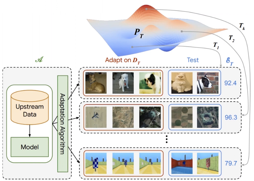
The primary goal is to create a general visual representation—a model that understands the visual world so well that it can be quickly adapted to solve any new visual task with very few examples. This is benchmarked using the Visual Task Adaptation Benchmark (VTAB), which evaluates a model’s performance across 19 diverse tasks after pre-training.
The Path to Vision Transformers
Before ViT, the research explored several avenues:
- Self-supervised and Self-supervised Semi-supervised Learning (S4L): These methods showed improvement but were significantly outperformed by the next step.
- Large-scale Supervised Pre-training (BiT – BigTransfer): The major breakthrough came from scaling up supervised pre-training using conventional ResNet (CNN) architectures. The key findings were:
- Be Patient: Training these large models on large data required immense compute and patience (e.g., 8 GPU-months), as performance gains were slow but steady.
- Scale Up Data: Using massive, weakly-labeled internal datasets (like JFT with 300 million images) was crucial.
- Scale Up Models: Larger datasets only showed significant benefits when paired with proportionally larger models.
This scaling approach demonstrated that with enough data and model capacity, CNNs could achieve state-of-the-art performance and robustness.
Vision Transformer (ViT) Architecture
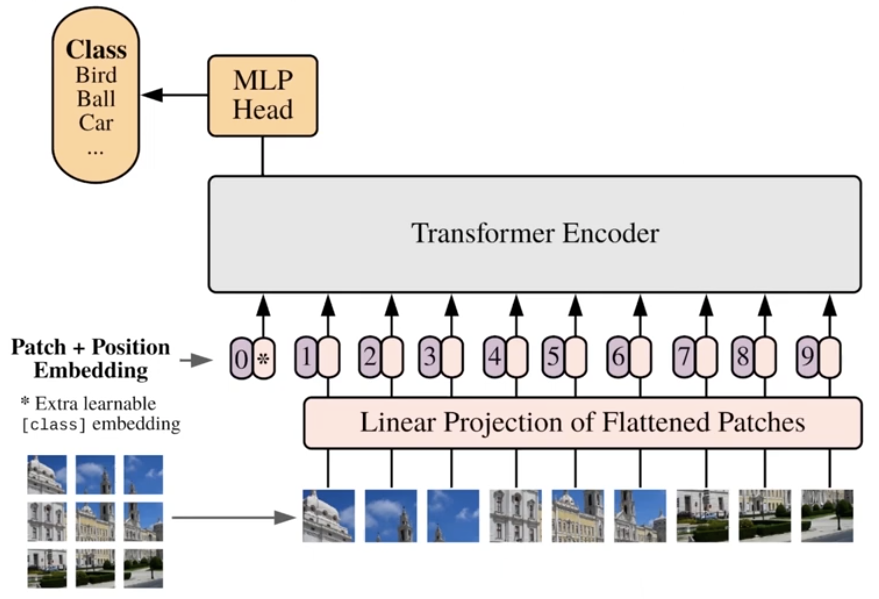
Inspired by the success of Transformers in NLP, the ViT applies the same architecture to images in the simplest way possible:
- Image Patching: An image is split into a grid of non-overlapping patches (e.g., 16×16 pixels).
- Linear Projection: Each patch is flattened and linearly projected to create a sequence of “image tokens.”
- Transformer Encoder: These tokens are fed into a standard Transformer encoder, exactly like word tokens in a language model. Learned positional embeddings are added to the tokens to retain spatial information.
The model is intentionally simple, with minimal “inductive bias” (pre-conceived assumptions about the data, like the locality inherent in CNNs).
Key Findings and Properties of ViT
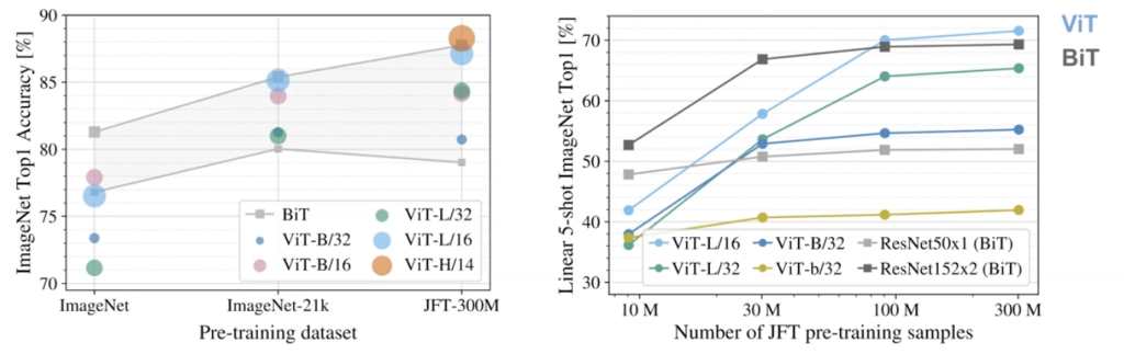
- Data is Key: When trained on smaller datasets like ImageNet (~1.3M images), ViT performs worse than comparable ResNets. However, when trained on massive datasets (100M-300M images), ViT starts to outperform the best ResNets. This suggests Transformers need large amounts of data to learn visual patterns that CNNs have as a built-in advantage.
- Learned Spatial Awareness: Despite having no built-in notion of 2D space, the model’s positional embeddings learn to represent the image’s grid structure.
- Attention Span: In early layers, the model’s attention heads learn a mix of local (nearby patches) and global attention. In later layers, the attention becomes almost exclusively global, looking across the entire image.
- Scaling Behavior: The best way to improve ViT is to scale its depth, width, and patch size together. Scaling up leads to better performance, especially on few-shot learning tasks.
Beyond the First ViT: Scaling and Evolution
- Are We Saturating?: No. A follow-up project scaled ViT to a 3 billion image dataset and found that performance continued to improve linearly on a log-log plot. This resulted in significant gains, achieving over 85% top-1 accuracy on ImageNet with just 10 examples per class.
- MLP-Mixer: To push the idea of reducing inductive bias further, researchers created the MLP-Mixer, which replaces the complex self-attention mechanism with simple MLPs. This architecture performs even worse on small data but surpasses ViT at a massive scale, reinforcing the idea that with enough data, simpler, more flexible architectures excel.
Papers
- A Large-scale Study of Representation Learning with the Visual Task Adaptation Benchmark
- Revisiting Self-Supervised Visual Representation Learning
- S4L: Self-Supervised Semi-Supervised Learning
- Big Transfer (BiT): General Visual Representation Learning
- An Image is Worth 16×16 Words: Transformers for Image Recognition at Scale
Decision Transformer: Reinforcement Learning via Sequence Modeling
The work explores framing Reinforcement Learning (RL) as a sequence modeling problem, leveraging the power and stability of Transformer architectures.
The Problem with Traditional Reinforcement Learning
While Transformers have revolutionized perception tasks (language, vision) with stable, scalable models, Deep RL policies have lagged behind:
- Smaller Scale: RL models typically have millions of parameters, compared to billions in large language models.
- Instability: Training is notoriously unstable, often relying on complex, sensitive dynamic programming methods (like the Bellman equation), leading to high variance in performance.
The goal of this research is to bring the stability and scalability of Transformers to the field of sequential decision-making.
The Decision Transformer: RL as Sequence Modeling
The core idea is to reframe RL not as a complex control problem, but as a simple sequence modeling or conditional generation task. The model, called the Decision Transformer, is intentionally simple:
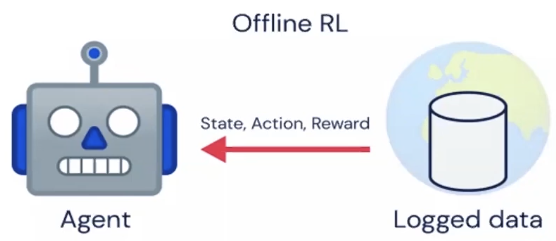
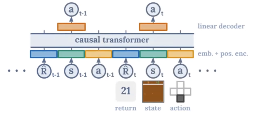
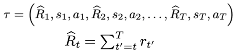
- Input: It takes sequences of past experiences from an offline dataset. A single “token” in this context is a triplet of (
return-to-go,state,action).- Return-to-Go (RTG): This is a crucial element. Instead of just the immediate reward, it’s the sum of all future rewards from the current timestep to the end of the trajectory. It acts as a conditioning signal, telling the model what level of performance to aim for.
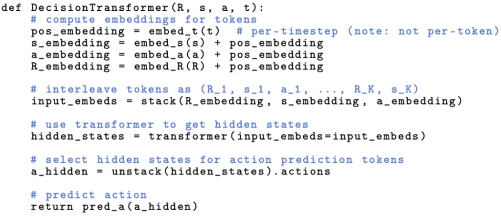
- Architecture: A standard causal Transformer (like GPT) is used. It processes the sequence of triplets and learns to predict the next action. Attention computed over context length K.
- Output: Sequence of predicted actions.
Code:
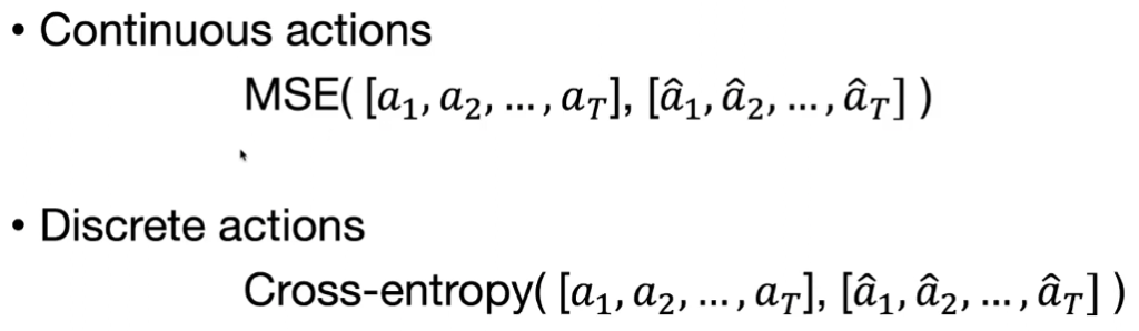
- Training: The model is trained with a simple supervised learning loss (e.g., mean squared error for continuous actions). This avoids the unstable Bellman updates common in RL, making training stable and predictable.
- Loss functions:
- Rollouts:
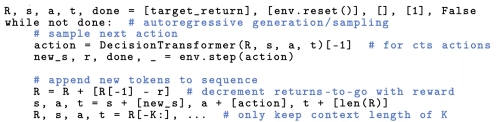
How It Works in Practice
- Training: The model learns to associate sequences of states and returns-to-go with the actions that produced them in the offline dataset.
- Evaluation (Rollout): To generate a policy, you give the model a target return (e.g., the return of an expert trajectory) and an initial state. The model then autoregressively predicts an action. You execute that action in the environment, get a new state and reward, update the return-to-go, and feed the new sequence back into the model to get the next action.
This process essentially turns policy generation into asking the model: “Given that I want to achieve this much total reward, what action should I take now?”
Key Findings and Advantages
- Competitive Performance: The Decision Transformer performs competitively with or even surpasses state-of-the-art model-free offline RL algorithms (like Conservative Q-Learning) on standard benchmarks (Atari, OpenAI Gym).
- Superior Long-Term Credit Assignment: It excels in sparse reward environments where the reward is only given at the very end. Because it’s conditioned on the final return from the start, it can better link early actions to distant outcomes, a major challenge for traditional methods.
- Return Conditioning as Multitasking: By changing the target return you provide at test time, you can elicit different behaviors from the model (e.g., a low-performing, cautious policy vs. a high-performing, expert policy) from a single trained model.
- Extrapolation: In some cases, the model can stitch together pieces of suboptimal trajectories from the dataset to produce a new trajectory that is better than any single one it saw during training.
- Data Efficiency: The model performs particularly well in low-data regimes compared to strong baselines like Behavior Cloning on only the best trajectories.
Future Directions
This work opens up several exciting avenues:
- Multimodality: Easily integrate different input types, like natural language instructions, with states and actions.
- Multitasking: Go beyond return conditioning to specify goals in more complex ways.
- Multi-agent RL: The model’s ability to handle long sequences is well-suited for modeling the behavior of other agents in an environment.
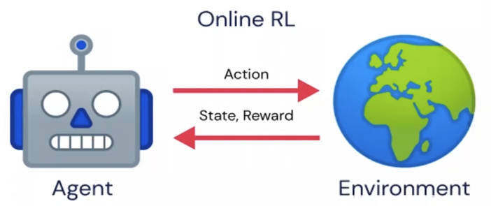
- Exploration: The biggest challenge is extending this framework to the online RL setting, where an agent must actively explore its environment. This is a non-trivial step and the main bottleneck for Transformers to completely take over RL.
Papers
- GPT-3: Language Models are Few-Shot Learners
- AlphaFold-2: Highly accurate protein structure prediction with AlphaFold
- ViT: An Image is Worth 16×16 Words: Transformers for Image Recognition at Scale
- Codex: Evaluating Large Language Models Trained on Code
- DALL-E: Zero-Shot Text-to-Image Generation
- Scaling Laws for Neural Language Models
- Decision Transformer: Reinforcement Learning via Sequence Modeling
Mixture of Experts (MoE) paradigm and the Switch Transformer
The lecture talks about scaling Transformers using the Mixture of Experts (MoE) paradigm, with a focus on the Switch Transformer. The core idea is to scale up models not by making them uniformly larger (dense), but by adding specialized sub-networks (experts) that are activated on a per-input basis.
Motivation: The Need for Sparsity
Scale is one of the most critical factors for improving model performance, as demonstrated by the “scaling laws” for neural networks. The conventional approach is to create larger dense models, where every input is processed by every weight in the model.
The alternative explored here is conditional computation via sparsely-activated models. This means that for any given input token, only a small subset of the model’s total parameters are used. This allows for creating models with a massive number of parameters without a proportional increase in the computational cost (FLOPS) for each token.
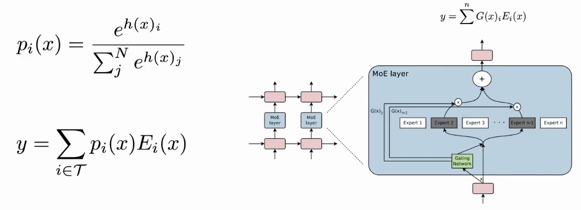
Mixture of Experts (MoE)
The standard Mixture of Experts (MoE) model operates by utilizing a “router” network to route each input token to a select number of “expert” sub-networks (e.g., the top 2). The final output is a weighted combination of the outputs from these selected experts.
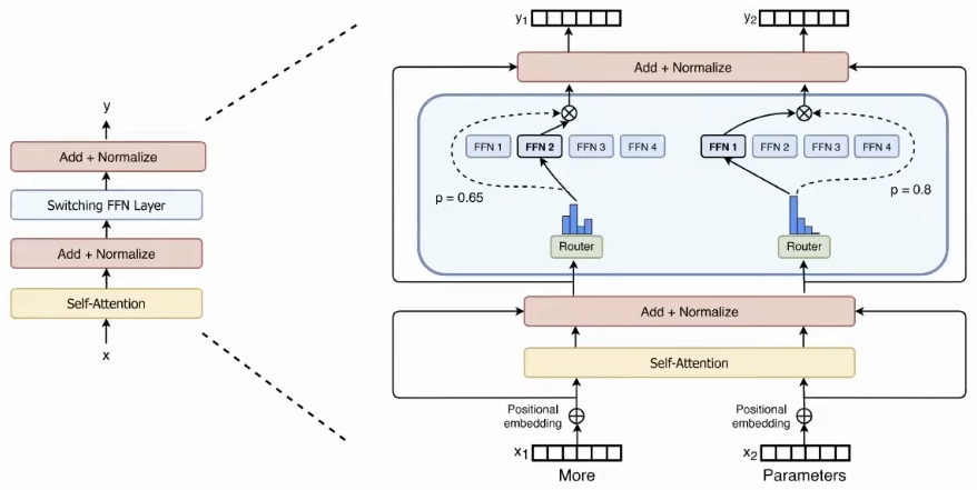
The Switch Transformer: A Simpler MoE
The Switch Transformer simplifies this design with key changes:
- Switching FFN Layer: Replace the Feed-Forward Network (FFN) layer in Transformer.
- Top-1 Routing: Instead of sending a token to multiple experts, each token is routed to only the single expert that the router network gives the highest probability.
This simplification proved to be more efficient. While a traditional MoE performs better when experts have a large buffer (high “capacity factor“), the Switch Transformer is more Pareto-efficient. It achieves a better speed-to-performance ratio, especially at lower capacity factors, which reduces communication, memory, and compute overhead.
Note: The expert capacity is the (static) maximum number of tokens each expert processes.
Key Techniques for Stable and Efficient Training
Several innovations were crucial for making these large, sparse models work effectively:
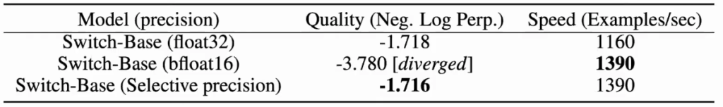
- Selective Precision: The models are trained in low-precision
bfloat16for speed, but this caused instability. The key insight was to cast just the router computation tofloat32. This negligible change in overall compute cost stabilized training significantly by preventing rounding errors in the router’s exponentiation function.
- Initialization and Regularization:
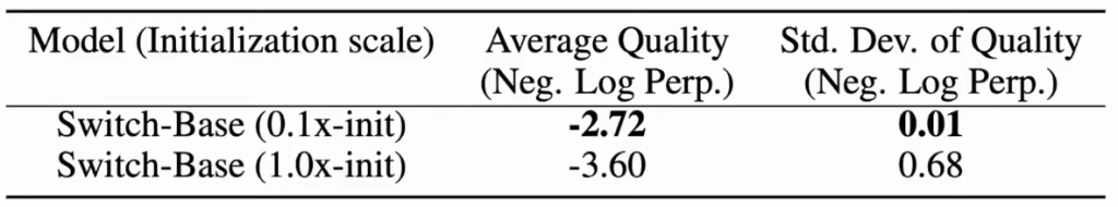
- The model’s weights were initialized at a smaller scale than standard Transformers, which drastically improved performance.
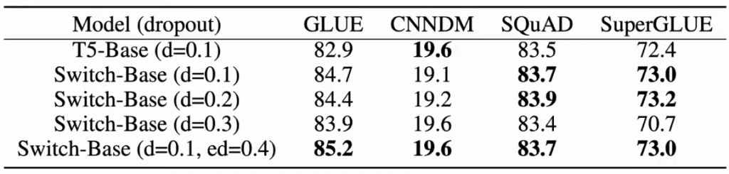
- To combat overfitting in these parameter-heavy models, a much higher dropout rate d was applied specifically to the expert layers during fine-tuning.
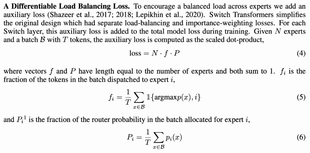
- Load Balancing: To ensure that all experts are utilized and computation is efficient on parallel hardware, an auxiliary loss was added. This loss encourages the router to distribute tokens roughly evenly across all the available experts during pre-training.
- Solution: A penalty for Imbalance
- To achieve this, we add a special “penalty” to the model’s main training objective. This penalty is the load-balancing loss.
- So, during training, the model has to learn to do two things at once:
- Get the main task right (e.g., predict the next word correctly).
- Keep the experts balanced to keep this penalty low.
- The Intuition Behind the Formula
- The formula
loss = N * f * Pmight look complex, but the idea is simple. It looks at two things:f(Fraction of tokens): This measures what actually happened. It’s the percentage of tokens in a batch that were sent to each expert. Ideally, if you have 8 experts, each should get about 12.5% of the tokens.P(Router’s confidence): This measures what the router wanted to do. It’s the average probability score the router assigned to each expert across all tokens. Ideally, the router should have roughly equal confidence in all experts.
- The formula
- The loss is calculated by multiplying these two things together. The model gets a high penalty if one expert receives a large fraction of the tokens (
fis high) AND the router was very confident about sending them there (Pis high). - To minimize this penalty, the model learns to adjust its router so that it doesn’t become overly confident in any single expert, which in turn causes the tokens to be distributed more evenly.
- Solution: A penalty for Imbalance
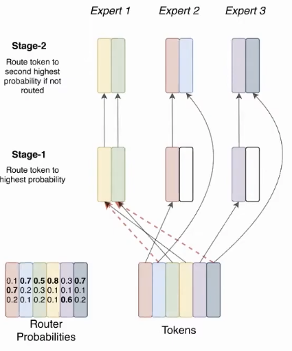
Modulate Expert Capacity with Capacity Factor
Problem: If too many tokens are route to a single expert then some tokens will be dropped.
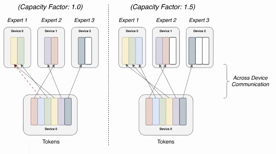
Solution: An attempt to avoid dropped tokens by sending to the next-best expert (if the preferred expert is at capacity). Empirically, this approach doesn’t work that well because tokens want to get to their highest probability expert.
Scaling, Performance, and Key Findings
- Scaling Speedup: Switch Transformers achieved up to a 7x speedup in pre-training time compared to a dense model with the same computational cost (T5-Base).
- Parameters vs. Compute: The researchers trained a massive 1.6 trillion parameter model called Switch-C that had significantly fewer FLOPS than smaller dense models. When fine-tuned, this model revealed a fascinating trade-off:
- It excelled on knowledge-heavy tasks (like TriviaQA).
- It underperformed on reasoning-heavy tasks (like SuperGLUE).
- This supports the hypothesis that parameters are for knowledge, and compute is for intelligence.
- Multilingual Performance: Sparsity was highly effective in multilingual settings, where experts could specialize in different languages, leading to significant speedups over dense multilingual models.
Making Sparse Models Practical: Distillation
A major drawback of MoE models is their large parameter count, making them difficult to deploy. The research showed that the knowledge from a large, pre-trained sparse model can be distilled back into a smaller, dense model. This process managed to retain ~30-40% of the performance gains from sparsity while reducing the parameter count by up to 99%, making the benefits accessible for practical applications.
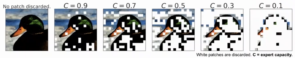
Future Directions: Vision and Adaptive Computation
The principles of MoE are also being applied to computer vision. In one compelling experiment, researchers used a capacity factor of less than 1.0, meaning the model was forced to drop most of the image patches and only process a small fraction (e.g., 10%) in the sparse layers. This worked remarkably well, demonstrating that the model can learn to identify and focus on the most important parts of an image, paving the way for more advanced adaptive computation.
Sparse Models for Computer Vision
- Sparse MoEs applied to Vision Transformer architecture (ViT)
- Images are partitioned into patches.
- Routing happens at the patch level.
- In-depth look into how trained routers work:
- Strong correlation between:
- Classes and expert choice in final layers.
- Patch position and expert in early layers.
- As expected, replacing router with random sampling hjurts perormance.
- Strong correlation between:
Priority Routing for Mixture of Experts
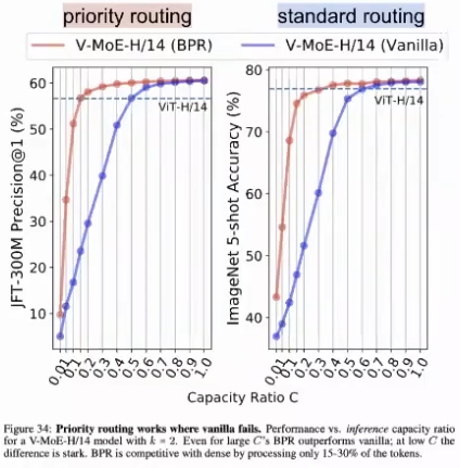
Ideas:
- Identify and prioritize “important” patches.
- Reduce the number of patches processed per expert (capacity C)
- Drop some patches (don’t process, but apply residual connection)
By reducing total amount of patches that are processed:
- Speed gains on inference and training.
- Performance largely preserved.
Papers
- Adaptive Mixtures of Local Experts
- Outrageously Large Neural Networks: The Sparsely-Gated Mixture-of-Experts Layer
- GShard: Scaling Giant Models with Conditional Computation and Automatic Sharding
- Switch Transformers: Scaling to Trillion Parameter Models with Simple and Efficient Sparsity
- End-to-End Human Pose and Mesh Reconstruction with Transformers
- V-MoE: Scaling Vision with Sparse Mixture of Experts
Reference
https://web.stanford.edu/class/cs25/past/cs25-v1
https://www.youtube.com/watch?v=BP5CM0YxbP8&list=PLoROMvodv4rNiJRchCzutFw5ItR_Z27CM&index=5
Leave a Reply