Object Detection – A Research Review

Introduction

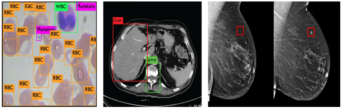
Object detection is a computer vision task that involves identifying and localizing objects within an image or video. It consists of two main steps:

Recognizing the types of objects present (such as cars, people, or animals).
Determining their precise locations by drawing bounding boxes around them.

The output of an object detection model for each identified instance is a tuple comprising a class label (c_i), the bounding box parameters (e.g., center coordinates, width, and height: x_i, y_i, w_i, h_i), and a confidence score (s_i) indicating the model’s certainty in the prediction.

Historical Milestones

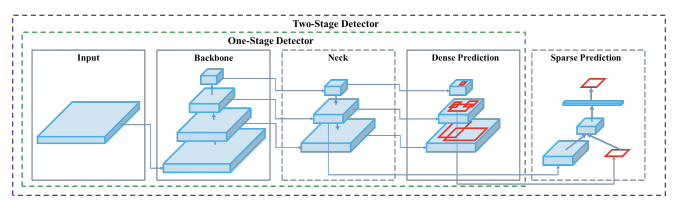
Two-Stage Detectors: Region-Based CNN Approaches

Early deep learning detectors followed a two-stage pipeline: first generate region proposals and then classify/refine them, favoring localization accuracy but typically at the cost of speed compared to one-stage methods.

R-CNN (Girshick, 2014):

Process: Uses an external algorithm (Selective Search) to generate ~2,000 region proposals. Each proposal is individually warped and fed through a CNN to extract features.
Components: Uses separate Support Vector Machines (SVMs) for classification and a linear regression model for refining bounding box locations.
Drawbacks: Extremely slow due to running a CNN for every single proposal. The training process is complex, involving multiple independent stages (CNN fine-tuning, SVM training, regressor training) that cannot be optimized together.

Fast R-CNN (Girshick, 2015):

Core Innovation: Processes the entire image through a CNN just once to create a shared convolutional feature map, drastically reducing computation.
RoIPooling: Introduces the RoIPooling layer to extract a fixed-size feature vector from the shared map for each region proposal, allowing different-sized regions to be processed.
Improvement: Combines the classifier and bounding box regressor into a single network that can be trained end-to-end (except for region proposals). This makes it significantly faster than R-CNN but still relies on an external proposal method like Selective Search.

Faster R-CNN (Ren et al., 2015):

Core Innovation: Introduces the Region Proposal Network (RPN), which integrates the region proposal step into the neural network itself.
Region Proposal Network (RPN): The RPN is a small network that slides over the shared feature map and uses predefined “anchor boxes” to predict object locations and “objectness” scores.
Improvement: By replacing the slow external proposal algorithm with a fast, learnable RPN, it creates the first truly end-to-end, unified object detection model, enabling real-time performance.

Cascade R-CNN:

Problem Solved: Addresses the “paradox of high-quality detection,” where training a detector with a high Intersection over Union (IoU) threshold leads to worse performance due to a mismatch between training and testing proposal quality.
Core Innovation: Employs a sequence of detector heads, each trained with a progressively higher IoU threshold (e.g., 0.5, 0.6, 0.7).
How it Works: During inference, proposals are refined sequentially by each head. The output of one stage becomes the input for the next, more specialized stage. This ensures each detector head is optimized for the quality of proposals it receives, leading to more precise final detections.

Other variants and extensions:

R-FCN (2016) used position-sensitive, fully convolutional heads to cut per-ROI computation.
Libra R-CNN (2019) rebalanced features and samples during training for better stability and accuracy.
Mask R-CNN (2017) extended Faster R-CNN with an instance segmentation branch, enabling detection + masks in one framework.

One-Stage Detectors: YOLO, SSD, and Beyond

To enable real-time detection, researchers developed one-stage detectors that eliminate the proposal stage and directly predict object class probabilities and bounding boxes on a dense grid of locations.

YOLO (Redmon et al., 2016):

Core Innovation: Frames object detection as a single regression problem, predicting bounding boxes and class probabilities directly from the full image in one pass.
YOLOv1 Process: The image is divided into an S×S grid. Each grid cell is responsible for predicting a fixed number of bounding boxes and class probabilities for objects centered within it. Non-Maximum Suppression (NMS) is used to clean up duplicates.
Key Evolutions:
- YOLOv2: Introduced anchor boxes for better shape prediction and batch normalization for stable training.
- YOLOv3: Used a deeper network (Darknet-53) and multi-scale predictions (predicting at three different feature map sizes) to significantly improve the detection of small objects.
- YOLOv4 & Beyond: Shifted to systematically integrating the best community techniques, categorized as “Bag of Freebies” (training-time boosts) and “Bag of Specials” (inference-time modules), leading to a rapid succession of highly optimized versions.

SSD (Liu et al., 2016):

Core Innovation: A single-shot detector that achieved high accuracy by making predictions from multi-scale feature maps at different depths of the network.
How it Works: It uses earlier, higher-resolution feature maps to detect small objects and later, lower-resolution maps to detect large objects.
Key Technique: Employs a set of default boxes (similar to anchors) at each location on the feature maps. To handle class imbalance, it uses hard negative mining, which only uses the most confident background predictions during training to prevent them from overwhelming the loss.

RetinaNet (Lin et al., 2017):

Problem Solved: Identified and fixed the primary reason one-stage detectors were less accurate than two-stage ones: extreme class imbalance, where the huge number of easy-to-classify background examples dominates the training process.
Core Innovation: Introduced the Focal Loss function, a dynamically scaled cross-entropy loss.
How it Works: The Focal Loss adds a modulating factor (1−p_t)^γ that down-weights the loss from easy, well-classified examples. This forces the model to focus its training effort on the sparse set of hard-to-classify objects.
Impact: When combined with a strong backbone (ResNet-FPN), Focal Loss allowed a one-stage detector to surpass the accuracy of contemporary two-stage detectors for the first time, closing the performance gap while maintaining high speed.

Anchor-Free Detectors

Researchers also explored anchor-free detectors that do not rely on predefined anchor boxes. These anchor-free approaches simplified the pipeline and avoided manual tuning of anchor sizes.

CornerNet (Law & Deng, 2018) and CenterNet (Zhou et al., 2019):

Localize objects by predicting keypoints (object corners or centers) rather than regressing anchor offsets.

FCOS (Tian et al., 2019):

Proposed a fully convolutional one-stage detector that predicts per-pixel objectness and regressions without anchors.
Achieving competitive accuracy (e.g. FCOS ~38–39% AP on COCO) with often simpler training.

Transformer-based Detectors

The most recent and profound paradigm shift in object detection has been the introduction of the Transformer architecture, a technology originally developed for and dominant in the field of Natural Language Processing (NLP). This new approach reframes the detection task in a way that eliminates the need for many of the hand-designed components, such as anchor boxes and Non-Maximum Suppression (NMS), that were central to previous CNN-based models.

DETR (DEtection TRansformer) (Carion et al., 2020):

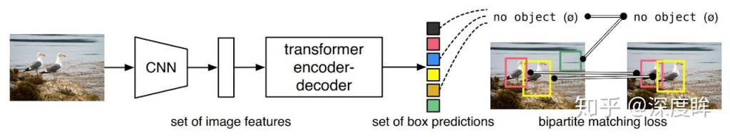
Core Innovation: Radically changes object detection by framing it as a direct set prediction problem. It’s the first model to use a pure Transformer architecture for detection.
How it Works:
- A CNN backbone extracts image features.
- A Transformer encoder-decoder processes these features. The decoder uses a small, fixed number of learned “slots” called object queries to probe the image features and ask, “What object is here?”
- Two feed-forward network (FFN) heads predict a class and a bounding box for each object query’s output.
Key Innovation: It completely eliminates the need for anchor boxes and Non-Maximum Suppression (NMS).
Loss Function: Uses bipartite matching (the Hungarian algorithm) to find a unique one-to-one assignment between its predictions and the ground-truth objects. The loss is calculated only on these matched pairs, which inherently teaches the model not to produce duplicate detections.
Drawbacks: The original DETR had very slow training convergence and struggled to detect small objects due to the high computational cost of its global attention mechanism.

Deformable DETR (Zhu et al., 2020):

Core Innovation: Replaces global attention with deformable attention. Instead of attending to every pixel, each query only attends to a small, learned set of key sampling points.
Impact: This reduces the computational complexity from quadratic to linear, allowing the model to process multi-scale feature maps. The result is 10x faster training convergence and significantly better accuracy, especially on small objects.

Conditional DETR, SMCA, and DAB-DETR:

Follow-up variants that refine the query–feature interaction and spatial focus to converge faster and boost accuracy, addressing DETR’s training efficiency and small-object issues.

Real-Time vs. High-Accuracy Detectors

Real-time focus

YOLOX (anchor-free + decoupled head + SimOTA) improved speed/accuracy trade-offs and became a strong industry baseline.

YOLOv7 introduced trainable BoF and E-ELAN design; strong accuracy at ≥30 FPS on common GPUs.

RT-DETR delivered the first real-time end-to-end transformer detector, eliminating NMS while competing with YOLO-family speed/accuracy; later variants (v2/v3) refined training supervision.

High-accuracy focus

Swin + Cascade

DINO (Zhang et al., 2022):

DINO combined multi-scale features with advanced training strategies to surpass 50% AP on COCO, rivaling the best CNN-based detectors while keeping the end-to-end Transformer formulation.

Conceptual Design Patterns

Backbones: CNNs (e.g., ResNet, CSP variants) and Vision Transformers; choice trades off capacity vs. latency.

Necks (multi-scale fusion): FPN (top-down + lateral), PANet (adds bottom-up paths), BiFPN (weighted bi-directional fusion, EfficientDet). These improve scale robustness with modest cost.

Heads: Coupled vs. decoupled classification/regression heads (common in YOLOX/RetinaNet) to reduce optimization interference.

Label assignment: Positive/negative sample selection is pivotal: ATSS adapts thresholds statistically; OTA/SimOTA formulate global assignment (optimal transport) or simplified dynamics.

Losses & post-processing: Beyond IoU: GIoU/DIoU/CIoU improve localization; Soft-NMS and DIoU-NMS can boost AP with little overhead.

Bag of Freebies and Bag of Specials

Bag of Freebies (Boosting Accuracy at No Inference Cost)

Data Augmentation

Its goal is to artificially increase the size and diversity of the training dataset by applying various transformations to the existing images. This exposes the model to a wider range of variations, improving its ability to generalize to unseen data and making it more robust.

Pixel-Level Augmentations: These modify the pixel values of an image.

Photometric Distortions: These alter the color and lighting properties of an image, including adjustments to brightness, contrast, hue, and saturation, as well as the addition of random noise. This helps the model become invariant to different lighting conditions.
Geometric Distortions: These transform the spatial properties of an image, such as random scaling (zooming), cropping, rotation, horizontal or vertical flipping, and translation (shifting). These techniques teach the model to recognize objects from different viewpoints and at different positions within the frame.

Image-Level Occlusion Augmentations: These techniques simulate object occlusion, forcing the model to learn from partial object views.

CutOut and Random Erasing: A random rectangular region of the input image is selected and its pixels are erased (e.g., set to zero or a mean value). This prevents the model from relying too heavily on any single salient feature of an object.
GridMask and Hide-and-Seek: These are extensions of CutOut that erase multiple rectangular regions in a structured or random grid-like pattern.

Augmentations Using Multiple Images: These methods create new training samples by combining information from two or more images.

MixUp: A new image is formed by taking a weighted linear interpolation of two images. The corresponding labels are also mixed with the same weights. This encourages the model to learn simpler linear relationships between samples.
CutMix: A patch is cut from one image and pasted onto another. The ground-truth label is then mixed proportionally to the area of the pasted patch. This has been shown to be a highly effective augmentation strategy.
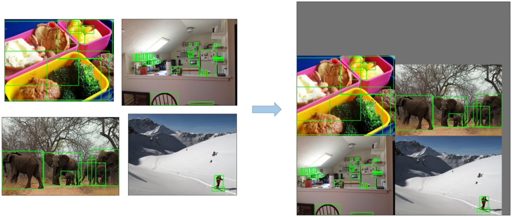
Mosaic Augmentation: A popular technique in the YOLO series, Mosaic combines four different training images into a single image. This allows the model to learn to detect objects in a much wider variety of contexts and at scales that might not be present in the original images.
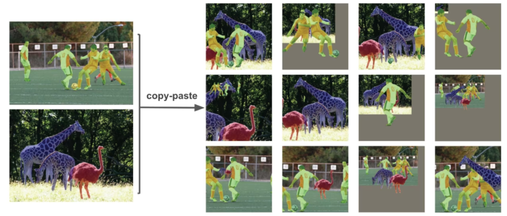
Copy-Paste: This technique, particularly useful for instance segmentation and rare object classes, involves segmenting objects from one image and pasting them onto another, often in a realistic manner. This can significantly increase the number of training instances for underrepresented classes.

Generative Augmentations: A more recent frontier involves using powerful generative models, such as Generative Adversarial Networks (GANs) or controllable diffusion models, to synthesize entirely new, diverse, and realistic training images, complete with bounding box annotations.

Loss Functions

The design of the loss function—the objective that guides the model’s learning—is a critical component of the BoF. A well-designed loss function can better align the training process with the final evaluation metric (mAP, which is based on IoU) and address inherent challenges in the training data.

For Classification:

Focal Loss: As detailed in the section on RetinaNet, this loss function effectively addresses the problem of extreme class imbalance between foreground and background examples by dynamically down-weighting the loss for easy, well-classified examples.

For Bounding Box Regression: Traditional regression losses like L1 or L2 (Mean Squared Error) do not directly correlate with the IoU metric used for evaluation. This has led to the development of a family of IoU-based losses.

IoU Loss: Directly optimizes the IoU. Its major drawback is that it produces a zero gradient for non-overlapping boxes, meaning the model cannot learn how to move the boxes closer together in such cases.
Generalized IoU (GIoU) Loss: Solves the zero-gradient problem by adding a penalty term that is minimized when the area of the smallest box enclosing both the predicted and ground-truth boxes is reduced. This provides a meaningful gradient even when the boxes do not overlap.
Distance-IoU (DIoU) Loss: Improves upon GIoU by adding a penalty term that directly minimizes the normalized distance between the center points of the two boxes. This leads to significantly faster convergence, as it provides a more direct optimization path.
Complete-IoU (CIoU) Loss: Extends DIoU by incorporating an additional penalty term that encourages consistency in the aspect ratio between the predicted and ground-truth boxes. CIoU often provides the best convergence speed and final regression accuracy.

Regularization

Regularization techniques are designed to prevent the model from overfitting to the training data, thereby improving its ability to generalize to new, unseen data.

Weight Decay (L2 Regularization): This is a standard technique that adds a penalty to the loss function proportional to the square of the magnitude of the model’s weights. It encourages the model to learn smaller, more distributed weights, which often leads to better generalization.

Label Smoothing: This technique addresses potential label noise and prevents the model from becoming overconfident in its predictions. Instead of using hard one-hot labels (e.g., ), it uses soft labels (e.g., [0.05, 0.95]). This small change can lead to improved robustness and calibration.

Dropout Variants for CNNs:

Standard Dropout: During training, this technique randomly sets the activations of a fraction of neurons to zero. This prevents neurons from co-adapting too much and forces the network to learn more robust and redundant features.
DropBlock: A more structured form of dropout designed for convolutional layers. Instead of dropping individual random neurons, DropBlock removes entire contiguous regions of a feature map. This is more effective at regularizing CNNs because activations in feature maps are spatially correlated.

Bag of Specials (Trading Minimal Cost for Significant Gains)

Feature Fusion

Feature fusion modules are designed to combine feature maps from different layers of the backbone network to create representations that are both semantically rich (from deep layers) and spatially precise (from shallow layers).

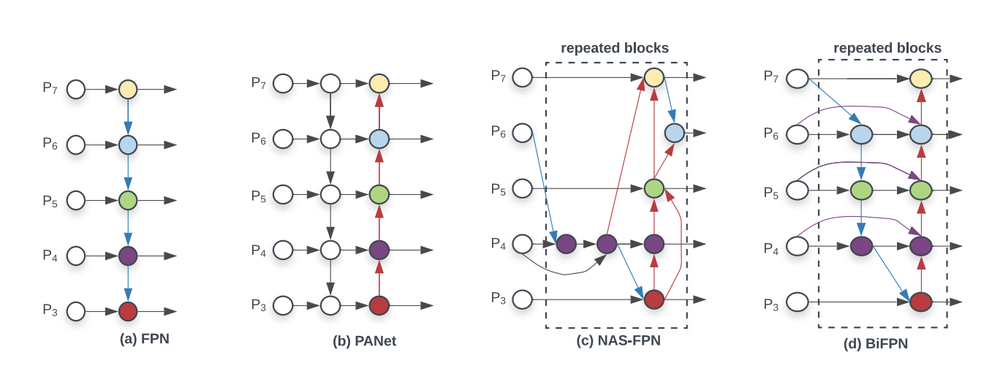
Feature Pyramid Network (FPN): The FPN is a foundational feature fusion architecture. It takes the standard bottom-up pathway of a CNN and augments it with a top-down pathway and lateral connections. The top-down pathway upsamples the semantically strong features from deeper layers and the lateral connections merge them with the high-resolution features from shallower layers, creating a pyramid of high-quality feature maps at multiple scales.

Path Aggregation Network (PANet): PANet enhances the FPN by adding an additional bottom-up feature aggregation path after the top-down path. This shortens the information path between the lowest layers and the topmost features, improving the propagation of fine-grained localization signals.

BiFPN, Rep-BiFPN: These are more advanced, weighted bidirectional FPNs that learn the importance of different input features and apply more efficient cross-scale connections.

Attention & Activations

These modules aim to improve the network’s learning capacity and focus.

Activation Functions (e.g., Mish): While ReLU is computationally cheap and effective, more advanced activation functions can offer performance benefits. Mish is a smooth, non-monotonic activation function (f(x)=x⋅tanh(softplus(x))) that can outperform ReLU. Its properties—being unbounded above (preventing saturation) and bounded below, along with its smoothness—can lead to better gradient flow and improved accuracy, albeit at a slightly higher computational cost.

Attention Modules: Attention mechanisms allow a network to learn to dynamically weight the importance of different features.

Squeeze-and-Excitation (SE) Module: This module focuses on channel attention. It learns to model the interdependencies between channels, adaptively re-calibrating the channel-wise feature responses by explicitly modeling which channels are more important.
Convolutional Block Attention Module (CBAM): CBAM sequentially infers attention maps along two separate dimensions, channel and spatial. This allows the network to learn “what” and “where” to focus in the feature maps, refining them for better representation.
Spatial Attention Module (SAM): This module specifically focuses on the spatial dimension, generating an attention map that highlights the most salient regions within a feature map, effectively teaching the network where to look.

Post-Processing

Standard Non-Maximum Suppression (NMS) is a greedy algorithm that can erroneously suppress correct bounding boxes in scenes with dense, overlapping objects. Advanced NMS variants are designed to be more robust.

Soft-NMS: Instead of harshly discarding any bounding box whose IoU with a higher-scoring box exceeds a threshold, Soft-NMS reduces its confidence score as a continuous function of the overlap. This allows it to retain valid detections in crowded scenarios.

DIoU-NMS: This variant modifies the NMS criterion by using the DIoU metric instead of the standard IoU. Since DIoU considers the distance between the centers of the bounding boxes, it is less likely to suppress a nearby but distinct object, which is a common failure case for standard NMS in occluded scenes.

Evaluation Protocols

Object detection is primarily a supervised learning task. This means that the dataset is composed of images and their corresponding bounding boxes, which serve as the ground truth.

Metrics:

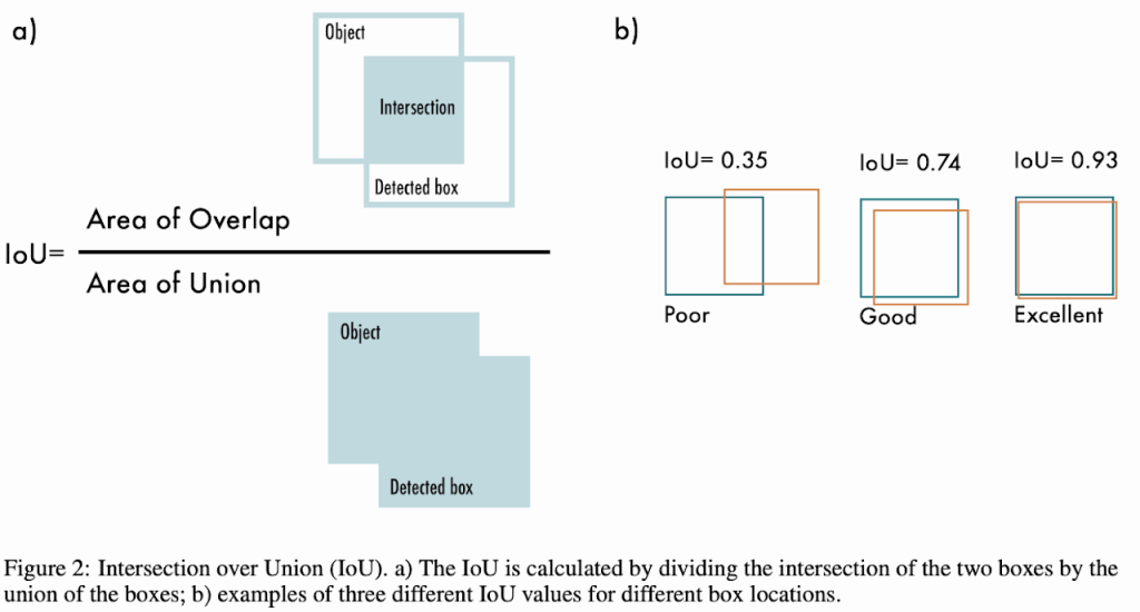
The Intersection over Union (IoU) or Jaccard index:
- Measures the overlap between predicted and reference labels as a percentage ranging from 0% to 100%.
- Higher IoU percentages indicate better alignments, i.e., improved accuracy.

COCO Mean Average Precision (mAP):
- Estimates object detection efficiency using both precision (correct prediction ratio) and recall (true positive identification ability).
- Calculated across varying IoU thresholds, mAP functions as a holistic assessment tool for object detection algorithms.

Reference

Papers:

[1] R. Girshick, “Rich feature hierarchies for accurate object detection and semantic segmentation,” in Proc. IEEE Conf. Comput. Vis. Pattern Recognit. (CVPR), 2014, pp. 580–587.

[2] R. Girshick, “Fast R-CNN,” in Proc. IEEE Int. Conf. Comput. Vis. (ICCV), 2015, pp. 1440–1448.

[3] S. Ren, K. He, R. Girshick, and J. Sun, “Faster R-CNN: Towards real-time object detection with region proposal networks,” in Proc. Adv. Neural Inf. Process. Syst. (NeurIPS), 2015, pp. 91–99.

[4] T.-Y. Lin, P. Dollar, R. Girshick, K. He, B. Hariharan, and S. Belongie, “Feature pyramid networks for object detection,” in Proc. IEEE Conf. Comput. Vis. Pattern Recognit. (CVPR), 2017, pp. 936–944.

[5] W. Liu et al., “SSD: Single shot multibox detector,” in Proc. Eur. Conf. Comput. Vis. (ECCV), 2016, pp. 21–37.

[6] J. Redmon, S. Divvala, R. Girshick, and A. Farhadi, “You only look once: Unified, real-time object detection,” in Proc. IEEE Conf. Comput. Vis. Pattern Recognit. (CVPR), 2016, pp. 779–788.

[7] T.-Y. Lin, P. Goyal, R. Girshick, K. He, and P. Dollar, “Focal loss for dense object detection,” in Proc. IEEE Int. Conf. Comput. Vis. (ICCV), 2017, pp. 2980–2988.

[8] H. Law and J. Deng, “CornerNet: Detecting objects as paired keypoints,” in Proc. Eur. Conf. Comput. Vis. (ECCV), 2018, pp. 734–750.

[9] X. Zhou, D. Wang, and P. Krahenbuhl, “Objects as points,” arXiv preprint arXiv:1904.07850, 2019.

[10] Z. Tian, C. Shen, H. Chen, and T. He, “FCOS: Fully convolutional one-stage object detection,” in Proc. IEEE Int. Conf. Comput. Vis. (ICCV), 2019, pp. 9627–9636.

[11] N. Carion et al., “End-to-end object detection with transformers,” in Proc. Eur. Conf. Comput. Vis. (ECCV), 2020, pp. 213–229.

[12] X. Zhu et al., “Deformable DETR: Deformable transformers for end-to-end object detection,” in Proc. Int. Conf. Learn. Represent. (ICLR), 2021.

[13] H. Zhang et al., “DINO: DETR with improved denoising anchor boxes for end-to-end object detection,” in Proc. Int. Conf. Learn. Represent. (ICLR), 2023.

[14] M. Tan, R. Pang, and Q. V. Le, “EfficientDet: Scalable and efficient object detection,” in Proc. IEEE Conf. Comput. Vis. Pattern Recognit. (CVPR), 2020, pp. 10781–10790.

[15] S. Zhang et al., “Bridging the gap between anchor-based and anchor-free detection via adaptive training sample selection,” in Proc. IEEE Conf. Comput. Vis. Pattern Recognit. (CVPR), 2020, pp. 9759–9768.

[16] Z. Ge, S. Liu, F. Wang, Z. Li, and J. Sun, “YOLOX: Exceeding YOLO series in 2021,” arXiv preprint arXiv:2107.08430, 2021.

[17] C.-Y. Wang et al., “YOLOv7: Trainable bag-of-freebies sets new state-of-the-art for real-time object detectors,” in Proc. IEEE Conf. Comput. Vis. Pattern Recognit. (CVPR), 2023.

[18] W. Zhao et al., “RT-DETR: Real-time detection transformer,” in Proc. IEEE Conf. Comput. Vis. Pattern Recognit. (CVPR), 2024.

[19] T.-Y. Lin et al., “Microsoft COCO: Common objects in context,” in Proc. Eur. Conf. Comput. Vis. (ECCV), 2014, pp. 740–755.

[20] N. Bodla, B. Singh, R. Chellappa, and L. S. Davis, “Soft-NMS—Improving object detection with one line of code,” in Proc. IEEE Int. Conf. Comput. Vis. (ICCV), 2017, pp. 5561–5569.

[21] Z. Zheng, P. Wang, W. Liu, J. Li, R. Ye, and D. Ren, “Distance-IoU loss: Faster and better learning for bounding box regression,” in Proc. AAAI Conf. Artif. Intell., 2020, pp. 12993–13000.

[22] P. F. Jaeger, S. Kohl, F. Bickelhaupt, F. Isensee, K. Maier-Hein, “Retina U-Net: Embarrassingly simple exploitation of segmentation supervision for medical object detection,” in Proc. Med. Image Comput. Comput.-Assist. Intervent. (MICCAI), 2018, pp. 171–180.

[23] C. F. Baumgartner et al., “nnDetection: A self-configuring method for medical object detection,” in Proc. Med. Image Comput. Comput.-Assist. Intervent. (MICCAI), 2021, pp. 530–539.

Le Phong Phu